Self-Backtracking

Abstract

The integration of slow-thinking mechanisms into large language models (LLMs) offers a promising way toward achieving Level 2 AGI Reasoners, as exemplified by systems like OpenAI's o1. However, several significant challenges remain, including inefficient overthinking and an overreliance on auxiliary reward models. We point out that these limitations stem from LLMs' inability to internalize the search process, a key component of effective reasoning. A critical step toward addressing this issue is enabling LLMs to autonomously determine when and where to backtrack, a fundamental operation in traditional search algorithms. To this end, we propose a self-backtracking mechanism that equips LLMs with the ability to backtrack during both training and inference. This mechanism not only enhances reasoning ability but also efficiency by transforming slow-thinking processes into fast-thinking through self-improvement. Empirical evaluations demonstrate that our proposal significantly enhances the reasoning capabilities of LLMs, achieving a performance gain of over 40 percent compared to the optimal-path supervised fine-tuning method.

Method

Under the standard Supervised Fine-Tuning (SFT) framework, we typically employ a dataset \(\mathcal{D}_{op} = \{(x_i, y_i)\}_{i \in [n_{op}]}\), where for reasoning tasks, \(y_i\) represents the natural language reasoning path representing the optimal solution. To enable the model to backtrack at appropriate times and positions, we introduce a backtracking dataset: \[\mathcal{D}_{back} = \{\left(x_j, \texttt{prefix}(y_j) \circ a_{err} \circ \langle \texttt{backtrack} \rangle\right)\}_{j \in [n]}.\] Here, \(\texttt{prefix}(y_j)\) denotes the prefix of the optimal solution \(y_j\), representing a partial solution; \(a_{err}\) signifies an erroneous action extended from the partial solution, which cannot lead to the correct answer; and \(\langle \texttt{backtrack} \rangle\) is a special token indicating that the model needs to backtrack from the current state. The final dataset is \(\mathcal{D}=\mathcal{D}_{op}\cup\mathcal{D}_{back}\).

Our self-backtracking technique consists of three main phases:

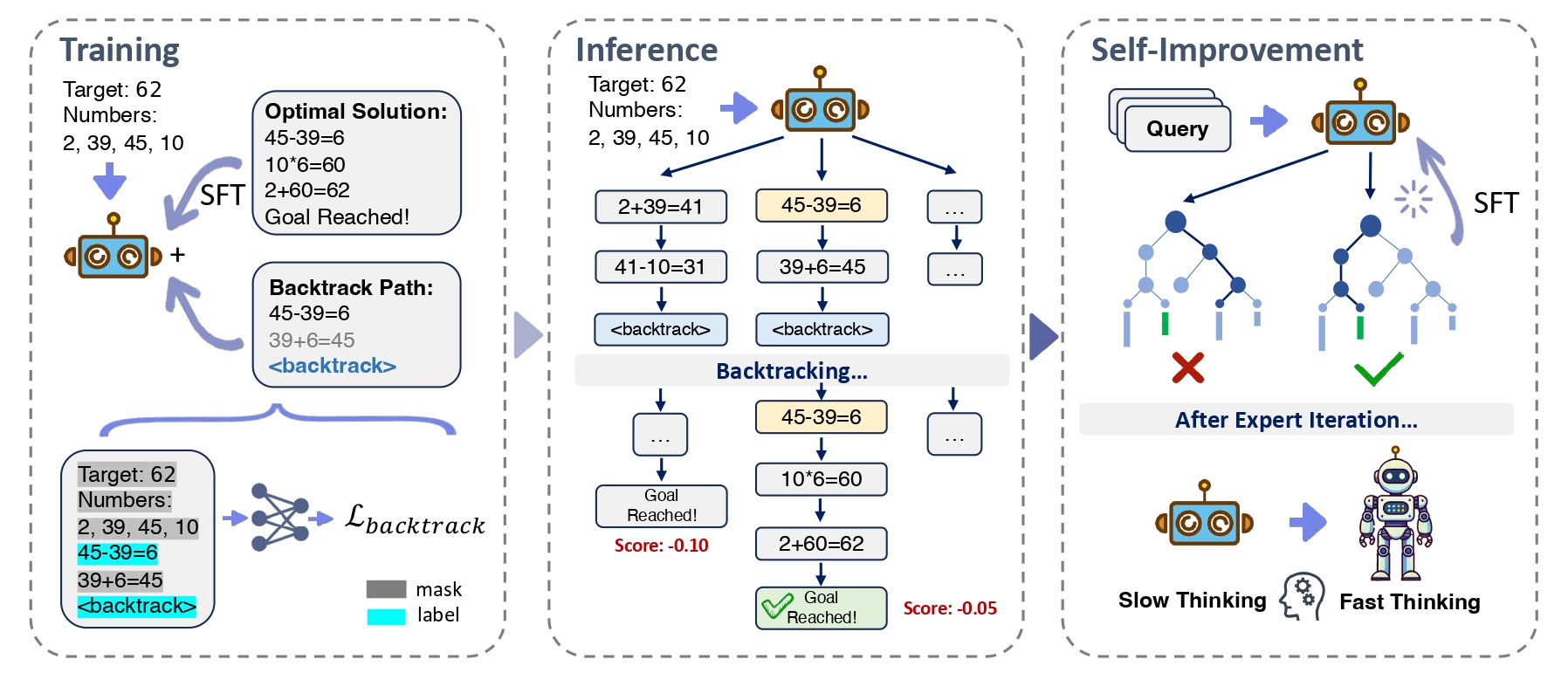
1. Training Phase

We train the model using a combination of optimal solution data and backtracking data:

\[ \mathcal{L}(\theta) = \mathcal{L}_{SFT}(\theta)+\mathcal{L}_{backtrack}(\theta) \]

The training loss function consists of two components: the supervised fine-tuning (SFT) loss and the backtracking loss. The backtracking dataset is constructed to help the model learn when and where to backtrack by introducing erroneous actions and a special backtrack token.

\[ \mathcal{L}_{backtrack}(\theta) = -\frac{1}{n_{back}}\sum_{j=1}^{n_{back}}\log p_{\theta}(\texttt{prefix}(y_j)|x_j) -\frac{1}{n_{back}}\sum_{j=1}^{n_{back}} \log p_{\theta}(\langle \texttt{backtrack} \rangle | x_j \circ \texttt{prefix}(y_j) \circ a_{err}) \]

The backtracking loss function, \(\mathcal{L}_{backtrack}(\theta)\), is crucial for training the model to recognize when its current reasoning path is suboptimal and to backtrack to explore alternative paths. It consists of two main components:

Partial Solution Prediction: This component encourages the model to predict partial solutions accurately given the input, ensuring that the model can generate correct reasoning steps up to a certain point.
Backtrack Token Prediction: This component focuses on the model's ability to predict the \(\langle \texttt{backtrack} \rangle\) token when it has deviated from the correct path. This helps the model learn to identify erroneous actions and backtrack appropriately.

Here, \(\texttt{prefix}(y_j)\) represents a partial solution, and \(a_{err}\) is an erroneous action. The \(\langle \texttt{backtrack} \rangle\) token indicates that the model should backtrack from the current state.

2. Inference Phase

During inference, we employ a novel search algorithm that considers both depth and breadth, consisting of three steps:

Expansion: Sample N predictions and categorize them
Backtracking: Process backtracking containing backtrack tokens
Selection: Choose the best reasoning path based on perplexity scores

This algorithm leverages the learned backtracking capabilities without requiring external reward models, maintaining controllable computational costs.

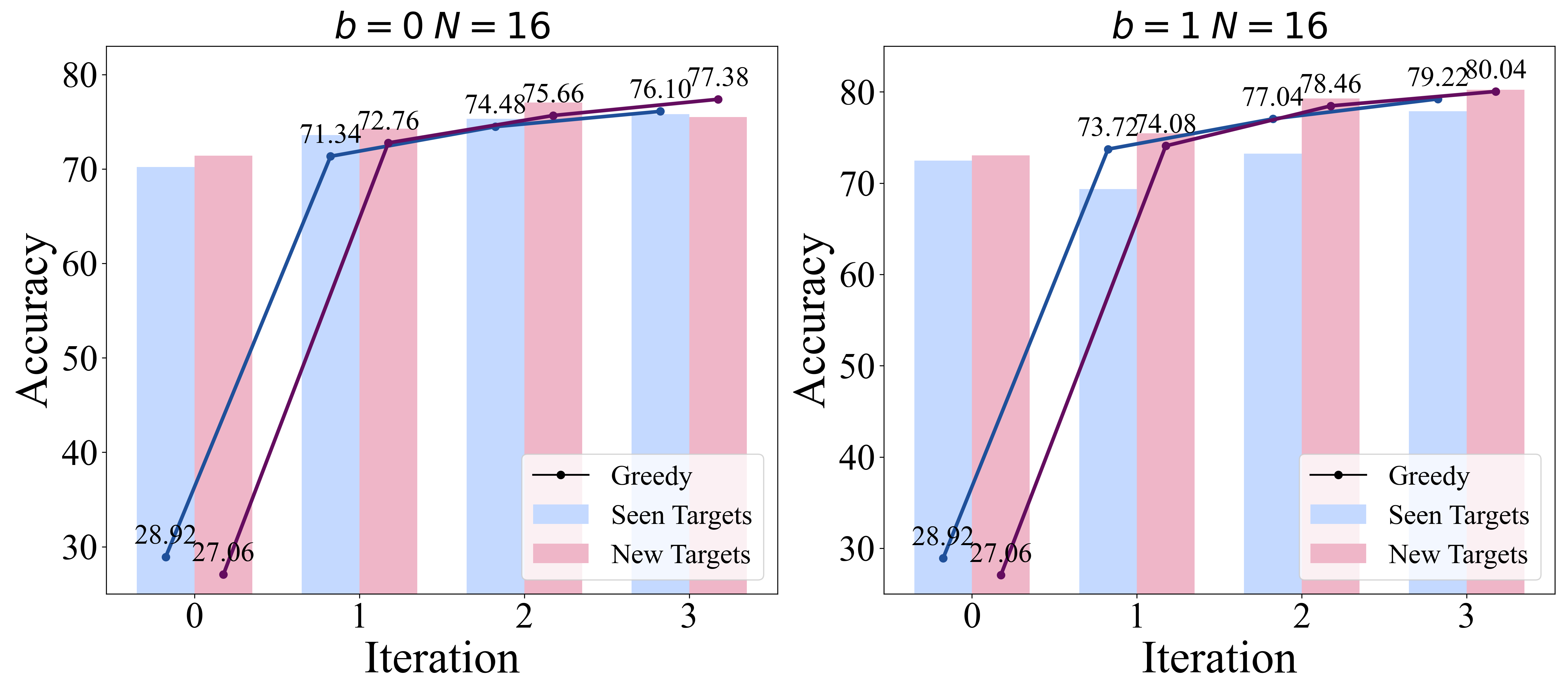
3. Self-Improvement Phase

In this stage we aim to transfer the model's slow thinking abilities to fast thinking through the self-improvement method. To achieve this, we employ an expert iteration strategy, which primarily consists of three steps: First, during the slow thinking data generation phase, we utilize the self-backtracking inference model to produce high-quality reasoning path data. Subsequently, in the expert screening phase, experts evaluate the generated data to select training samples suitable for the fast thinking model. In our experiment, we quantify the model's accuracy using an evaluator. Finally, in the fast thinking model training phase, the selected high-quality data is used to train the fast thinking model by SFT. Through this iterative optimization, we get continuous enhancement in the performance of the fast thinking model.

Results

We employ the Countdown task as our principal experimental framework to rigorously evaluate the reasoning capabilities of our self-backtracking approach. This task extends the traditional 24 Game by necessitating that LLMs strategically combine a provided set of input numbers using fundamental arithmetic operations—addition, subtraction, multiplication, and division—to achieve a predefined target number. The complexity of the task stems from its expansive search space, which rigorously tests the models' ability in reasoning the correct path.

Main Results

We present the accuracy of various methods across different models for the countdown task. Overall, the self-backtracking technique demonstrates a significant improvement over the baseline of greedy search after SFT, with enhancements of approximately 40% on Llama3.2-1B and over 30% on Llama3.2-3B.

Analysis

We conduct experiments by varying the \(b\) and \(N\), and generate performance curves under different \(b\) values as \(N\) increases, as illustrated in Figure 2. The results demonstrate that the performance of BoN initially increases and then decreases with larger \(N\), which we attribute to the reward hacking. On the contrary, our method exhibits a consistent improvement with increasing \(N\), eventually stabilizing, indicating a clear test-time scaling law in breadth. Furthermore, when backtracking is permitted (\(b=1\)), the performance improves more rapidly with \(N\) and achieves a higher overall performance, underscoring the necessity of backtracking.

Further experiments demonstrate that our algorithm achieves self-improvement through expert iteration. Employing self-backtracking with configurations b=0, N=16 and b=1, N=16 on two base models and datasets respectively, we filtered correct reasoning paths from inference outputs for SFT. Figure 3 presents three-round improvement results, where bars indicate test performance using our algorithm (slow thinking) and lines represent greedy search (fast thinking). Each iteration brings moderate gains (1-2%)

We conduct experiments to analyze the error types for different \(b\) and \(N\). There are four error types: not reached target, invalid step format, incorrect result in step, and unknown numbers in step. The experimental results shown in Figure 4 demonstrate that our method progressively reduces the proportion of "Not reached target" errors by expanding the search scope. As the parameter \(N\) increases, the model explores more nodes. Allowing more backtracking provides the model with additional opportunities for error correction and retreat, thereby enhancing the probability of finding the correct answer.

Citation

@article{selfbacktracking,
  title={Step Back to Leap Forward: Self-Backtracking for Boosting Reasoning of Language Models},
  author={Xiao-Wen Yang and Xuan-Yi Zhu and Wen-Da Wei and Ding-Chu Zhang and Jie-Jing Shao and Zhi Zhou and Lan-Zhe Guo and Yu-Feng Li},
  journal={arXiv preprint arXiv:2502.04404},
  year={2025}
}